In the 1930’s, two indepentent mathematicians, Leonid Kantorovich and Wassily Leontief were busy producing something that would be overlooked for decades: The true and practical application of linear equations in an increasingly modern, increasingly mechanical world. While their groundbreaking work was overlooked by peers like Alan Turing and John Von Neumann, both of whom would have profound impact on the world of mathematics and computer science, Kantorovich and Leontief’s work would nontheless be just as important in our modern age as Turing’s and von Neumann’s.
By 1949, Wassily’s work would finally pay off, with Dr. Leontief creating a program for the Mark II that would permanently change the way in which computers were used by economists, business professionals, and individuals who use applied mathematics. He wrote a program, mathematically rigorous but converted to the Instruction Set Language of the Mark II, that took a number of linear equations and solved the model in 52 hours. This was the first instance of a mechanical computer being able to solve such large models and while trivial for programmers today, it was a feat that would have quiet, but profound impacts on the world of economics.
Meanwhile, in the USSR, under the heel of the slowly dying Stalin and the powerstruggle that would ensue from this, Kantorovich’s work would be left mostly obscure and underused. Regardless, both gentlement would share the 1973 Nobel Prize for Economics for their research into linear modeling of economics data.
Variables, Equations, and Systems of Equations
Such problems have a number of variables. If you recall, a variable is any unknown and we usually represent them with numbers like $x$ and $y$. We can use these variables in functions like
$$y=mx+b$$Which is you recall is our simple formula for a linear equation, where $m$ is our coeffecient and $x$ is a variable. This is pretty simple and we can do all sorts of analysis on just this formula alone (which we would call pre-algebra and algebra 1). However, once we start to add in a bunch of variables, it gets pretty crazy:
$$2x + \frac{2}{3}y+27z = 34$$To help us just a tiny bit, bucause we could have more than 26 variables, let’s rename $y$ and $z$ to $x_2$ and $x_3$ respectively. But also, what if we have several equations all using these same variables:
$$\begin{cases} 5x_1 + 12x_2 = 42 \\ x_1 + 5x_2 = 12 \end{cases}$$The question is this Can we find what the value of $x_1$, $x_2$, and $x_3$ could be, where each of the 3 equations are true?
This is called a system of equations and is surprisingly important throughout many areas, from math to finance, from accounting to chemstry, every field relies on some ability to balance and convert equations. Being able to understand how to handle these will set us up for what we will learn later in this series.
Properties of Linear Systems of Equations
There are some general properties that we should be aware of regarding linear systems of equations:
First, a linear system of equations may have 1 of 3 solutions
1. No solution at all
Consider the following system:
$$\begin{cases} x+y+z = 0 \\ x+y+z=1 \end{cases}$$There is no way to determine a solution that would resolve both equations. Therefore this system has no solution at all. Solving one would ultimately fail the other and vice versa.
Another example is the following:
$$\begin{cases}y = -2x-1 \\ y = 3x-2 \\ y = x+1 \end{cases}$$If you were to graph these examples, you would see that they do not all converge at a single point, rather they all meet each other separately at different places. They have no solution that resolves each of them together. As a result, there is no solution for the system.
2. One Unique Solution
Our original system has exactly one solution. If you were to graph it in a calculator or a site like Desmos, you could see that the lines intersect together at exactly one point. We’ll look at how to prove this mathematically soon.
3. Infinite Solutions
Consider this: $x = y$ and $y=x$
There are an infinite number of solutions that could solve this system.
I want to point out a word I used above. Convergence is something we will be using while studying AI, Optimization, and Computational Complexity. You can think of a solution to a system as being where lines of a graph converge together to a single point, to many points, or do not converge at all. While we will explore this later on down the road, I felt it was best to signpost this concept now, rather than later.
Solving Linear Systems of Equations
Let’s go back to our initial problem:
$$\begin{cases} 5x + 12y = 42 \\ x + 5y = 12 \end{cases}$$I’ve rewritten it into our (x,y) form, which will make sense very soon. If you recall from algebra 1, we can take x and y variables and convert them into the point-slope formula:
$$\begin{cases} y = -\frac{5}{12}x + \frac{21}{6} \\ y = -\frac{1}{5}x + \frac{12}{5} \end{cases}$$And use that to manually graph our lines. Or, alternatively, you can use desmos like a normal person:
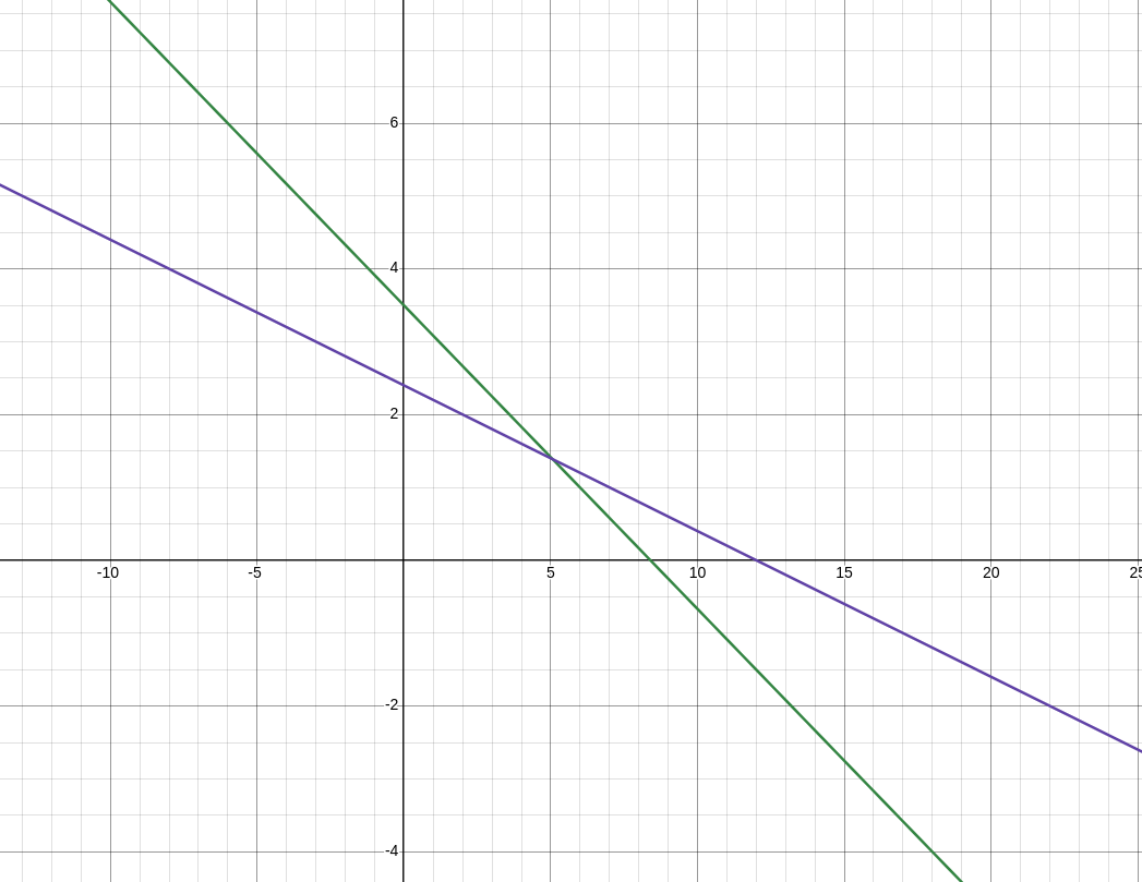
See where the two lines cross? This is our solution. As there is only one, we would call it a unique solution.
But what if we don’t want to graph it? The Mathematician Carl Gauss figured out a method for solving these sorts of problems that resulted in the exact same solution set as the ones above:
- We can moves the rows around
- we can replace a row by adding it to a multiple of another row
- We can multiply a row by a constant number that isn’t zero
What is key about these actions is that they are always the same as the row we are working on, ever single time. We’ll prove it over the next couple of examples below.
Solving our simple, 2-equation system:
We can see that if we take -5 and multiply it to the second row, we get $-5x-25y=-60$ If we were to add that result to the first row, we would get $-13y = -18$. Now, you might be thinking “Man, no way this works. It can’t possibly also be in our linear system, right?” Remember: We can verify that if it converges with the other lines on the graph, it is valid.
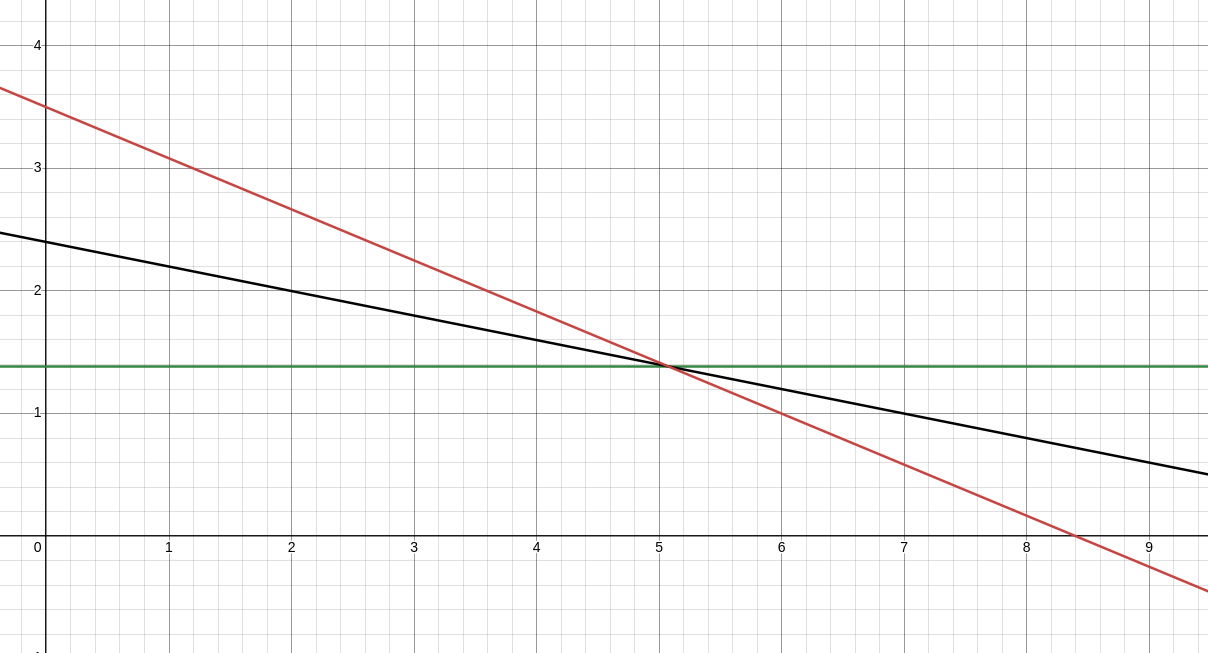
It works y’all. $y$ does in fact, $=-\frac{18}{13}$.
We can use this fact that $y = -\frac{18}{13}$ to find x. Just take 1 equation (we’ll do the second one because it is easiest), and substitute y for $\frac{18}{13}$. Do the arithmatic again, and you wind up with $x = \frac{66}{13}$
We’ll prove it to be true one more time:
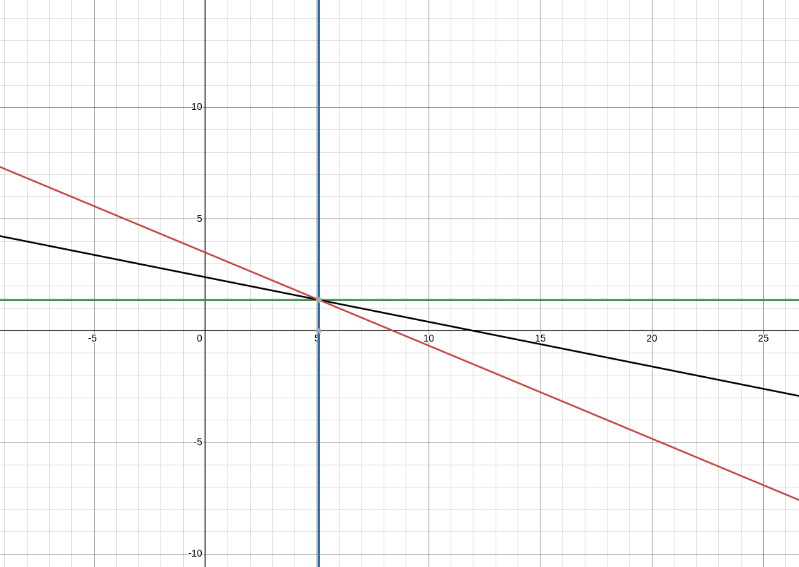
And voila! We have our solution set: $[x = \frac{66}{13}, y = \frac{18}{13}]$
Question: What if we have a LOT of variables?
Recall at that the beginning, I spoke about our friend Wassily having literally HUNDREDS of varables and HUNDRES of linear equations. What do you do when it isn’t quite so simple?
In the next article, we will look at Matrices, how to use them with linear systems of equations, and their properties.